


 96 / 352

92
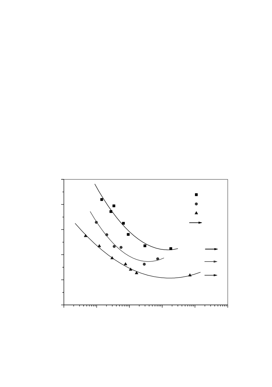
Other examples of metallic response to cyclic loading in this regime are also interes-
ting, like the behaviour of an aluminum alloy 2219-T85 (Fig. 5), showing a
S
max
versus
log
N
plot, with the supporting data shown /12/. This is a typical S-N diagram, showing
the fitted curve as the actual data that support the diagram. This is the currently required
approach for representing this type of information in the handbook /12/.
Plastics and polymeric composites are interesting materials for different responses un-
der mechanical loading, including dynamic excitation. The nature of hydrocarbon bon-
ding results in substantially more hysteresis losses under cyclic loading and a greater
susceptibility to frequency effects. An example of
S
-
N
results for a variety of materials is
given in Fig. 6. Also, different specifications are used for fatigue testing of plastics /13/.
The plastics industry also employs tests to determine a "static" fatigue response, which is
a sustained load test similar to a stress-rupture or creep test of metallic materials.
In application, this method is in its simplest form for steels in a neutral environment.
The task is to compare the
S
a
determined in the part to a
S
a
vs.
N
curve at the necessary
R
value. Acceptable safe-life, infinite-life situation exists if the applied
S
a
is less than the
fatigue limit. In a slightly more complex scenario, the
S
m
, S
a
pair applied in a component
is compared to the properly determined Goodman line on a Haigh diagram with two
possible results: on or under the Goodman line indicate an acceptable safe-life, infinite-
life situation, and results above the Goodman line indicate a finite-life situation that can
be managed if the general boundary conditions of the method are not abused.
10
3
10
4
10
5
10
6
10
7
10
8
0
100
200
300
400
500
Stresses are based
on net section
Stress ratio
0.500
0.050
-0.500
Runout
Maximum stress, MPa
Fatigue life, cycles
Figure 5: Best-fit S/N curves for notched, 2219-T851 aluminium alloy plate in longitudinal
direction, with stress concentration factor
K
t
= 2.0