


 100 / 352

96
10
1
10
2
10
-3
10
-2
10
-1
10
0
10
1
10
2
10
3
10
4
K
c
or K
Ic
final failure
Threshold
da/dN = C(
Δ
K)
n
Region 3:
Rapid
unstable
crack
growth
Region 2:
Power law
behaviour
Region 1:
Slow crack
growth
Δ
K
th
da/dN, nm/ciklus
Δ
K, MPa m
1/2
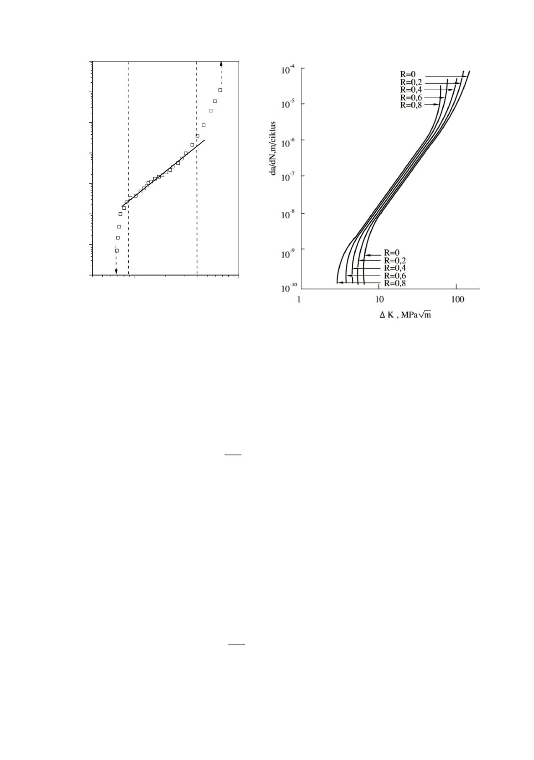
Figure 8. Asymptotic behaviour of
da
/
dN
vs.
ΔK
plot for 13 CrMo 4 4 steel at either end
and a linear portion in the central part /16/
Figure 9. The influence of
R
value on the fatigue
crack growth characteristics of a steel /17/
The crack length (
a
) increases with the number of fatigue cycles,
N
, when a
component or a specimen containing a crack is subjected to cyclic loading, if the load
amplitude (
ΔP
), load ratio (
R
), and cyclic frequency (
v
), are held constant. The crack
growth rate,
da
/
dN
, increases as the crack length increases during a given test and in
structure. The
da
/
dN
is higher at any given crack length at higher load amplitudes. Thus,
the following functional relationship can be derived from these observations:
(
)
R,
da
f P,a
dN
ν
⎛ ⎞ = Δ
⎜ ⎟
⎝ ⎠
(4)
where the function
f
is dependent on the geometry of the specimen or component, the
crack length, the loading configuration, and the cyclic load range. This general relation is
simplified with the use of the
ΔK
parameter as summarized below.
In 1963, Paris and Erdogan /18/ published an analysis with sufficient fatigue crack
growth rate (FCGR) data, deriving a correlation between
da
/
dN
and the cyclic stress
intensity parameter,
ΔK
. They argued that
ΔK
characterizes the magnitude of the fatigue
stresses in the crack tip region, characterizing the crack growth rate in agreement with the
relationships of Eq. (4). The parameter
ΔK
accounts for the magnitude of the load range
(
ΔP
) as well as the crack length
a
and geometry. Later studies /19/ has confirmed the
findings of Paris and Erdogan. The data for intermediate FCGR values can be represented
by the simple mathematical relationship, commonly known as the Paris equation:
(
)
n
I
da C K
dN
⎛ ⎞ = ⋅ Δ
⎜ ⎟
⎝ ⎠
(5)
where
C
and
n
are constants that can be obtained from the intercept and slope,
respectively, of the linear log
da
/
dN
versus log
ΔK
plot (Figs. 8 and 9).