


 189 / 352

185
Figure 10: Fracture surface of the specimen in the tilt stage on scanning electron microscope
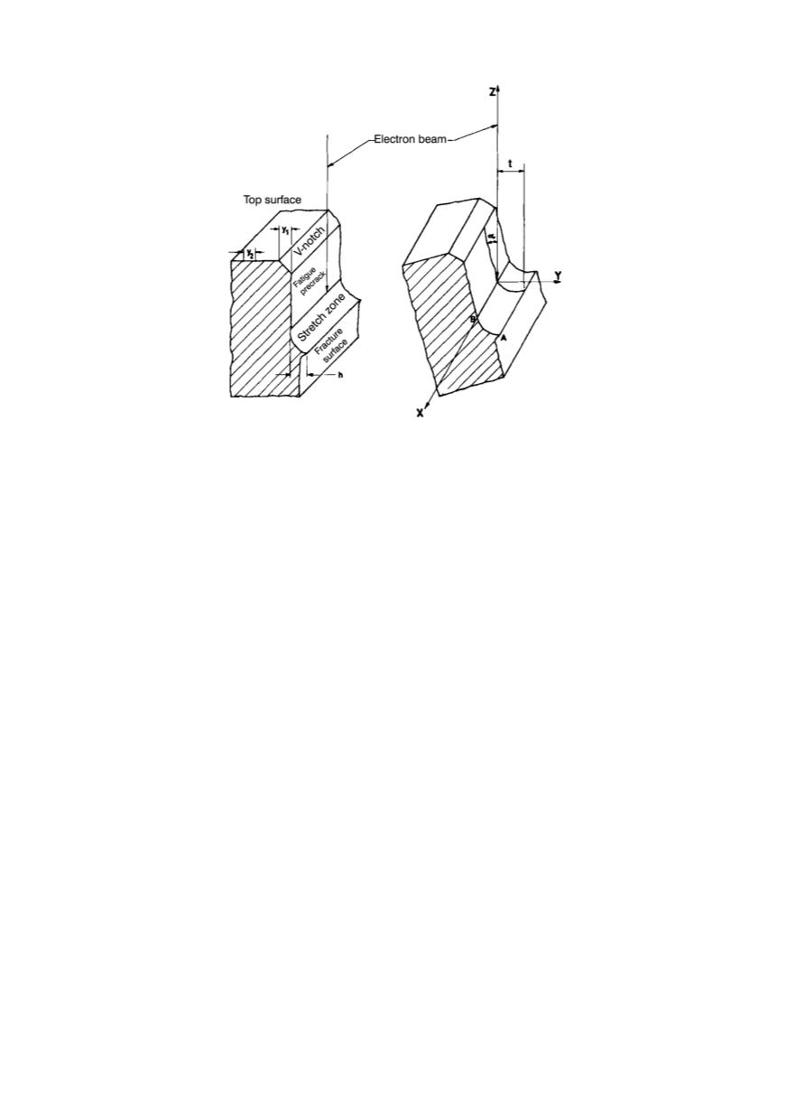
Visual examination of the highly magnified specimen, Fig. 11, gives the impression that
the stretch zone was uniform in the specimen midthickness. However, after measuring the
stretch-zone dimensions
w
and
t
, as discussed, it was obvious that the magnitude of these
values, as well as the magnitude of
h
, vary across the crack front. A typical variation of
w
,
t
,
and
h
across the specimen thickness is shown in Fig. 12. Although the stretch zone appears
uniform macroscopically, the variation in local microstructure and alteration in local
deformation characteristics as the crack tip blunts leads to differences in
w
and
t
values and
hence, in the magnitude of
h
.
The experimental measurements /10/ were made on high strength Mo-Nb micro-
alloyed steel NIOMOL, with 0.06% C (Fig. 13). The investigation was carried out on a
welded joint, and the results presented here are the measurements made on 10 mm wide
samples from the heat-affected-zone (HAZ). Seven fractographs were made by SEM,
which were then used to measure the width and the depth of the stretch zone/11/. Five
measurements were made per each fractographs, using Texture Analysis System, i.e. TAS
plus. Typical variation in the measured
w
,
t
and
h
in performed experiments is presented
in Fig. 14.
6.2. Fracture toughness obtained measuring stretch zone width and depth
The method for obtaining the J integral by measuring the stretch-zone width (SZW) is
based on the fact that SZW is equivalent to the critical virtual crack extension (
Δ
a
cr
) prior
to the onset of ductile tearing, a vertical line drawn at
Δ
a
= SZW. The J corresponding to
the intersection of this vertical line with the J-resistance curve is taken as
J
SZW
, Fig. 15.
For determination of J from the SZD, two methods were used.
In the first method, the CTOD calculated as per standard, was plotted against
Δ
a
, and
a line at
δ
= 2SZD is drawn to intersect the
δ
-
Δ
a
curve. The
Δ
a
value corresponding to
the intersection was labelled
Δ
a
cr
. The intersection of
Δ
a
cr
on the corresponding J-
Δ
a
curve is labelled
J
SZD
, Fig. 16.a. In the second method, the J -
δ
data are plotted, and a
vertical at
δ
= 2SZD is drawn. Intersection on J -
δ
curve is labelled
J
SZD
, Fig. 16.b.