IFMASS10

184

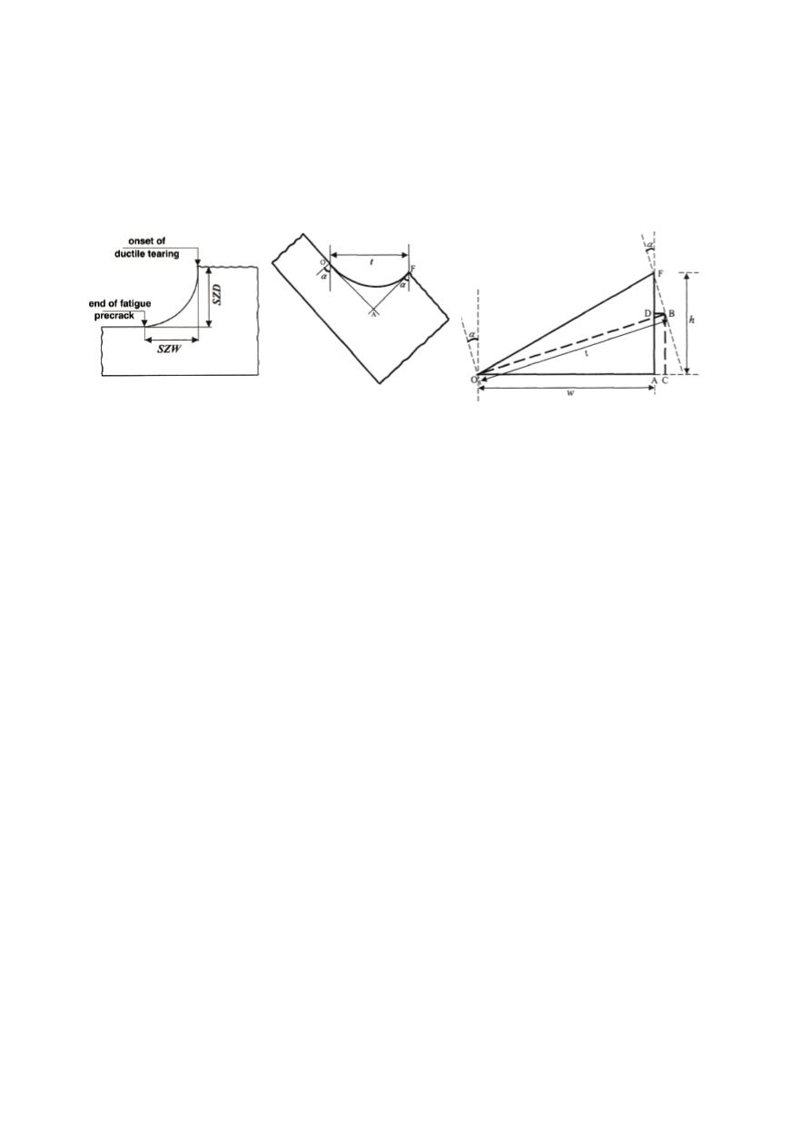
Using the identities specified above, the SZD of the stretch zone produced during

fracture can be calculated starting from values of

and

From the aforementioned scheme, it can be seen that if an error in accuracy is made

when identifying the true plane of fracture, the error in the calculation of

is given by the

product of the angular error between the true and actual reference frames and the stretch-

zone width (SZW). Similarly, the error made in the determination of

is equal to the

product of angular error and

a. Normal view

b. Tilted view

c. Normal and titled views (a. and b.)

Figure 9. Schematic view showing the geometric inter-relationship between the untilted and tilted

configurations of the stretch zone dimensions

6.1. Practical measurements of stretch zone geometry

The fractured surfaces were first extracted from the tested specimens and placed on the

stage of the scanning electron microscope (SEM), aligning the plane of fracture to be

normal to the electron beam, Fig. 10. This is ensured by measuring the size of a linear

feature of known length, like the notch.

At tilt position fixed to 0°, a representative stretch feature was recorded with a suffi-

ciently high magnification to be able to identify local features within the stretch zone,

while making sure that the whole width of the stretch zone was contained in the field of

view. In order to demarcate the stretch zone limits easily, efforts were made to ensure that

a good contrast was achieved.

Secondly, the SEM stage was tilted so that the fracture surface was rotated through

45° about an axis through the crack front, and the features recorded at the same

magnification. While tilting, it was important to ensure that there was no lateral shift of

the specimen, in order to view the same area of fracture surface previously examined.

Whilst it is true that the fracture features of the steels provide excellent contrast to

confidently demarcate the stretch zone, establishing the actual end of the stretch zone was

nonetheless difficult in the 0-deg tilt condition, due to the near vertical relief in this

region. Correspondence with features in the 45° tilted view, in which the end of the

stretch zone was more easily discernible, was therefore sought for identification of

stretch-zone limits. Such features are marked as A, B, and C in the fractographs, Fig. 11,

obtained in testing HSLA steel of 800 MPa nominal strength. As shown in Fig. 9,

and

were measured from tracings of the start and end of the stretch zones in 0° and 45° tilt

images on transparency grids. The correspondence between

and

was ensured through

identifiable features in both tilt conditions. Both halves of the specimens were measured

at least 30 times along the thickness direction. From each measurement of

and corres-

ponding

, the

value of the SZD was calculated using Eq. (3).