
312
TOT
S
K K K
σ
= −
(5)
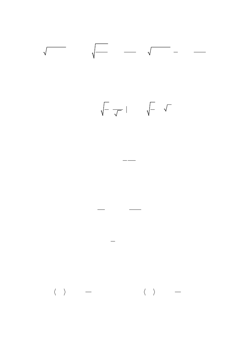
With constant
σ
and
S
the integrals are easy to evaluate and the two
K
-factors become
j
i
i
j
i
1
1
2
(
)
2
cos
(
) cos
S
c R
c
c
K
c R K S
S c R
c R
c R
σ
σ π
π
π
π
−
−
⎡
⎤
+
⎛
⎞
⎛
⎞
=
+
=
=
+
⎜
⎟
⎜
⎟
⎢
⎥
+
+
⎝
⎠
⎝
⎠
⎣
⎦
(6)
These two stress intensity factors remain in equilibrium
K
σ
=
K
S
during the process of
loading up to the point of incipient fracture. The function
K
σ
2
can be thought of as a
“driving force”, which forces the crack to open up, while
K
S
2
represents material
resistance. It is noted that
K
S
reduces to zero for a vanishing length of the cohesive zone.
For a physically important case of
R
being small compared to the crack length
c
the
second equation in (6) assumes a simple form
[ ]
i
i
i
(
)
0
2
2 2
R
S
S const
R c
Sd
K
S R
λ
π
π
λ
=
=
=
∫
(7)
Variable
λ
represents the distance measured backwards from the outer edge of the
cohesive zone. In this limiting case the cohesion modulus does not depend on the crack
size. It is expressed in terms of the magnitude of the cohesive stress and the length
R
.
Equating Eq. (7) with fracture toughness
K
c
and inverting the equation produce the
ubiquitous result
i
2
2
8
c
K R
S
π
=
(8)
This formula defines the characteristic length parameter as determined through the
cohesive model of fracture. Three essential variables are related via this simple equation,
which is valid only when
R
<<
c
. Otherwise, Eq. (6) must be used to define the length of
the cohesive zone as a function of stress
S
and the crack size
c
.
Next the finiteness condition employed, which with (6) reads
i
1
cos
0
2
c
S
c R
σπ
−
⎛
⎞
−
=
⎜
⎟ +⎝
⎠
(9)
With
Q
denoting non-dimensional loading parameter,
Q
=
πσ
/2
S
, one can solve Eq.
(9) for the length of the cohesive zone, namely
i
sec 1
R Q
c
= −
(10)
For small
Q
the right hand side reduces to ½
Q
2
, and Eq. (10) reduces to Eq. (8).
3. DISCRETIZATION OF THE COHESIVE CRACK MODEL
In order to account for the discrete nature of fracture process all
K
-factors discussed
above need to be replaced by their averages. Applying the scheme
0
0
0
0
1/2
1/2
2
2
,
,
0
0
1
1
c a
c a
S
S
S
c c a
c c a
c
c
K K
K dc
K K
K dc
a
a
σ
σ
σ
+
+
+
+
⎡
⎤
⎡
⎤
→ =
→ =
⎢
⎥
⎢
⎥
⎣
⎦
⎣
⎦
∫
∫
(11)
we proceed to evaluate the averages defined in (11). Symbol
a
0
denotes the fracture
quantum, which is used as a normalization constant for the length-like variables
X
and
R
,
i
0
0
/
/
X c a R R a
=
=
(12)


